Box Filter
D_x Convolution
D_y Convolution

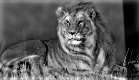
Grayscale Image
This blog explores image filtering techniques, frequency analysis, and multiresolution blending. We'll cover convolution operations, edge detection, hybrid image creation, and advanced blending techniques using Gaussian and Laplacian pyramids.
Here are the two implementations of 2D convolution:
We see that the two implementations as well as the scipy.signal.convolve2d function (when set to 'same' mode) all give the same output, but the speeds are significantly different with scipy taking a few seconds, 2d for loop in the tens of seconds, and 4d for loop in the multiple minutes when ran on test images.
Here are some images that we used this function on:
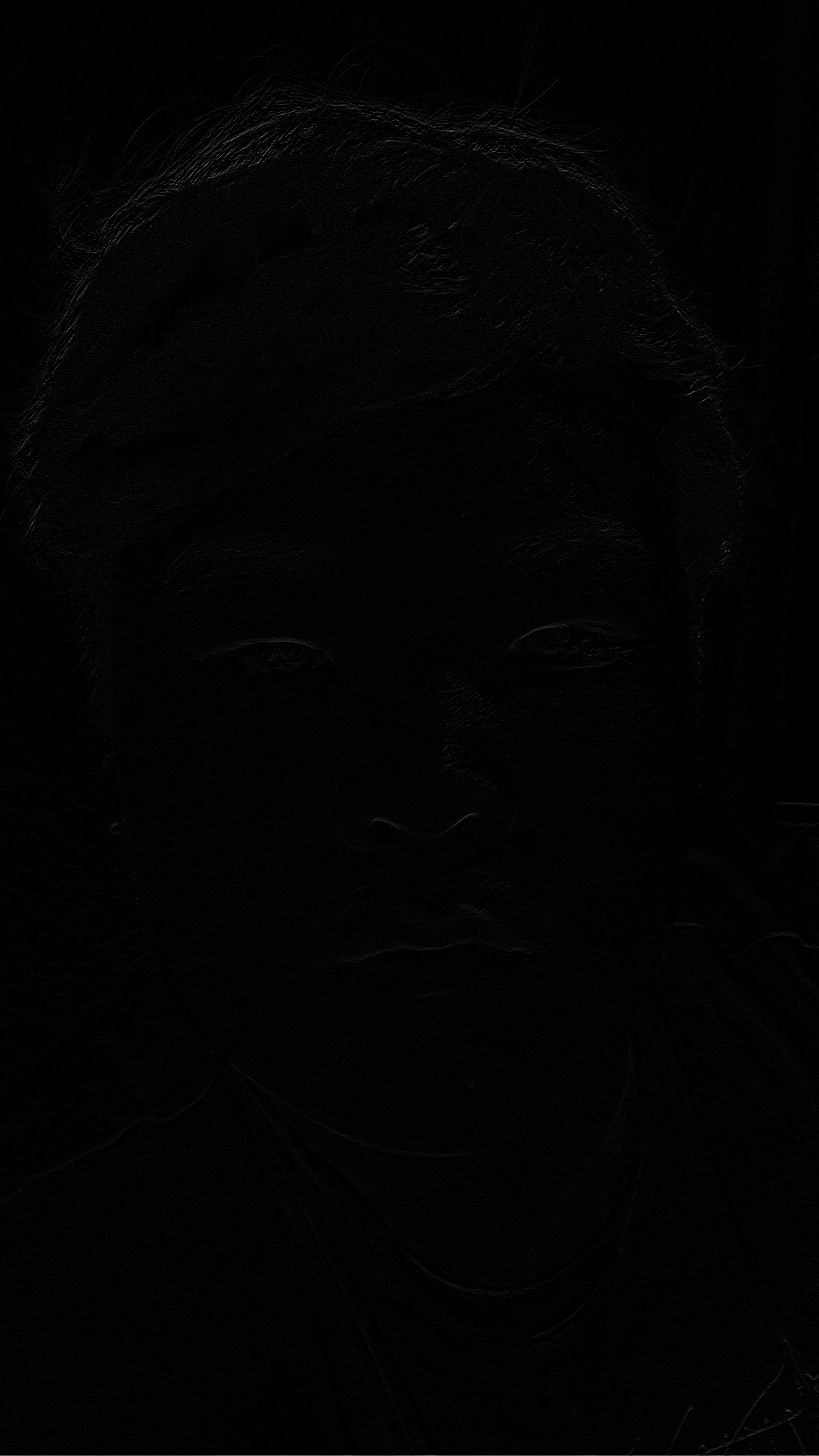
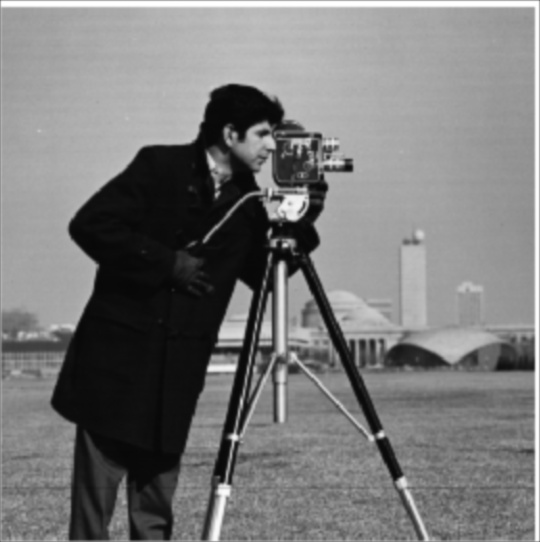
Here is the original cameraman image:

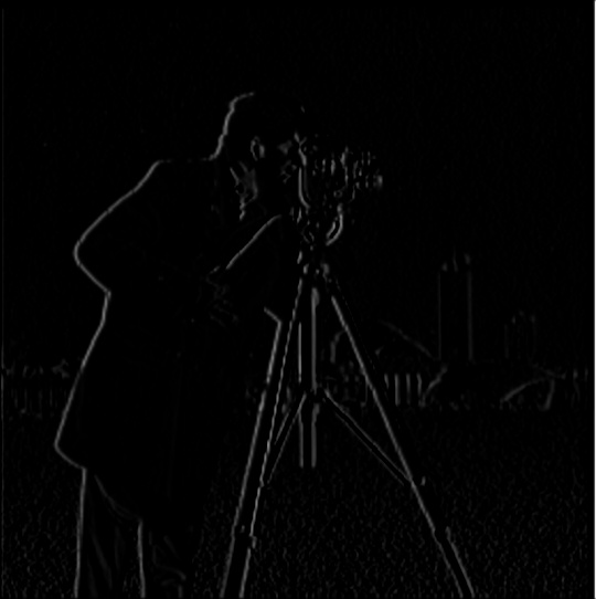
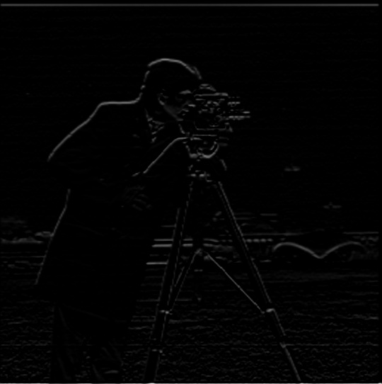
Here are the results when we run a convolution with d_x and d_y which are the finite difference operators on the cameraman image:
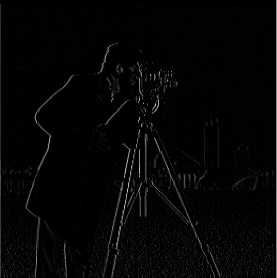
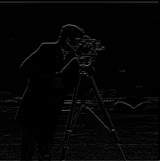
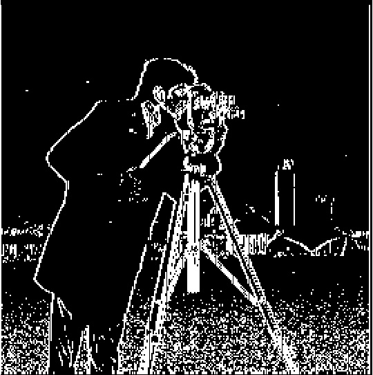
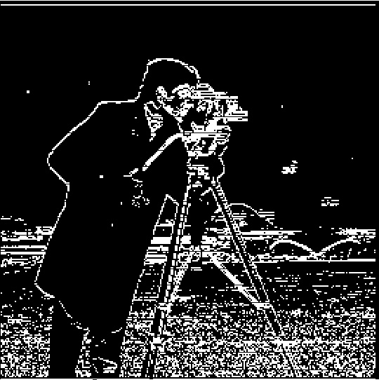
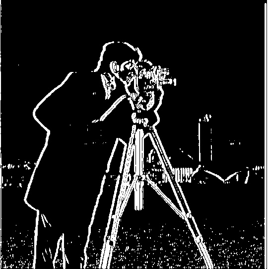
This doesn't show much so instead, we check different possible thresholds for the edges to make a binary plot. The threshold that we found was most useful was about 15. This was chosen as a higher threshold did not show the tower in the background whereas a lower threshold showed little specs in the sky which is shown in the following images:
Here are the results when we run a convolution with the gaussian filter:
We further check the partial derivatives of the gaussian filter:
We see that the partial derivatives of the gaussian filter are very similar to the finite difference operators, which is expected.
We also verify that this can be done with a single convolution, which is possible since convolutions are associative, using something like the following code:
We also show the output of the binary plots here:
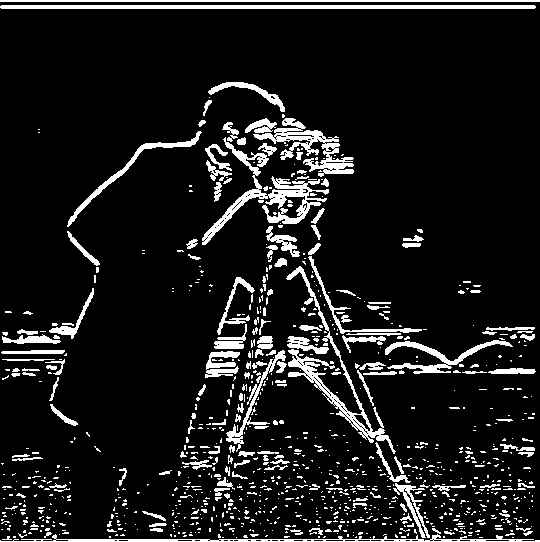
We see that the output is much smoother than the original because the gaussian filter helps reduce the noise in the image.
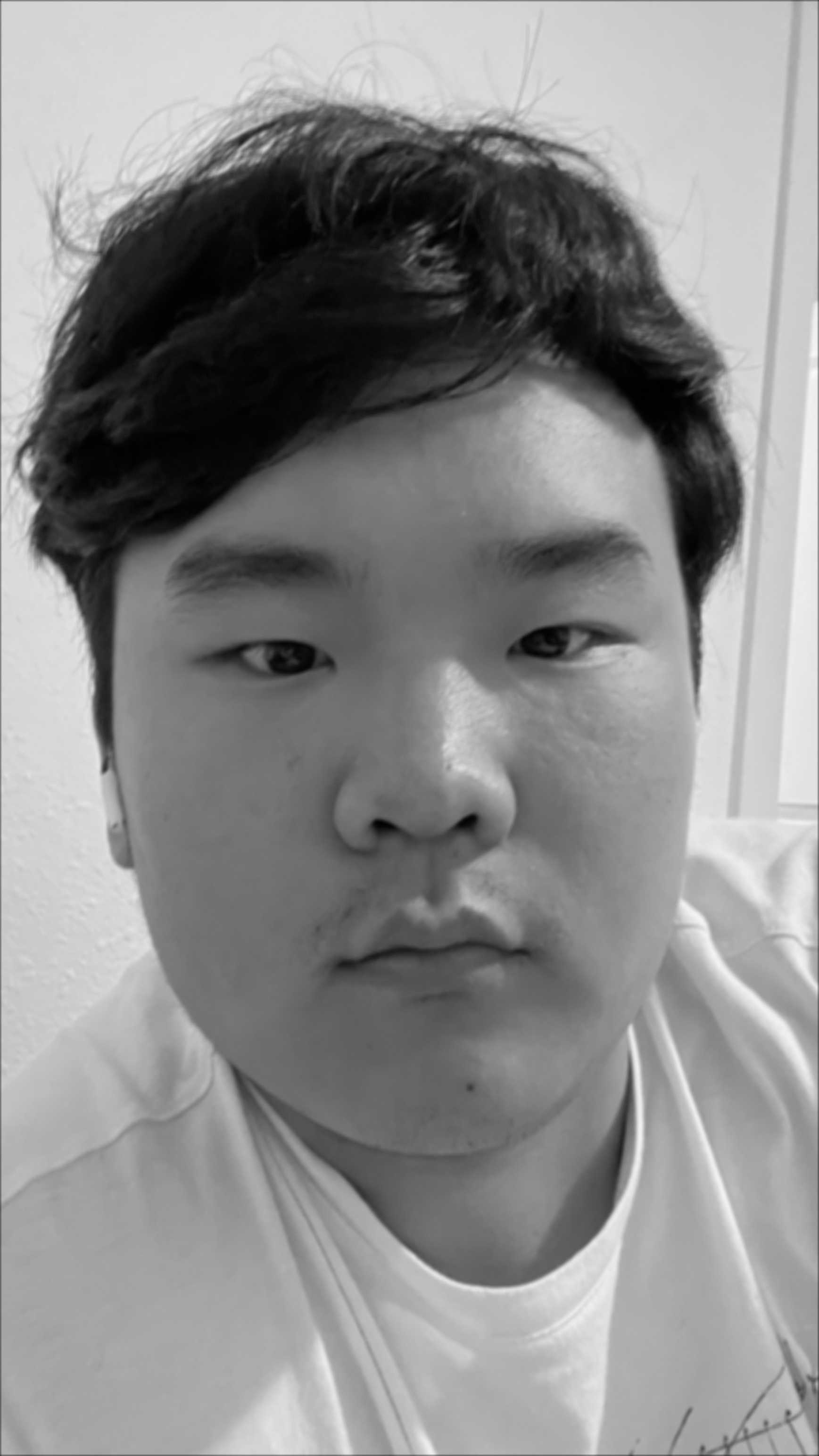
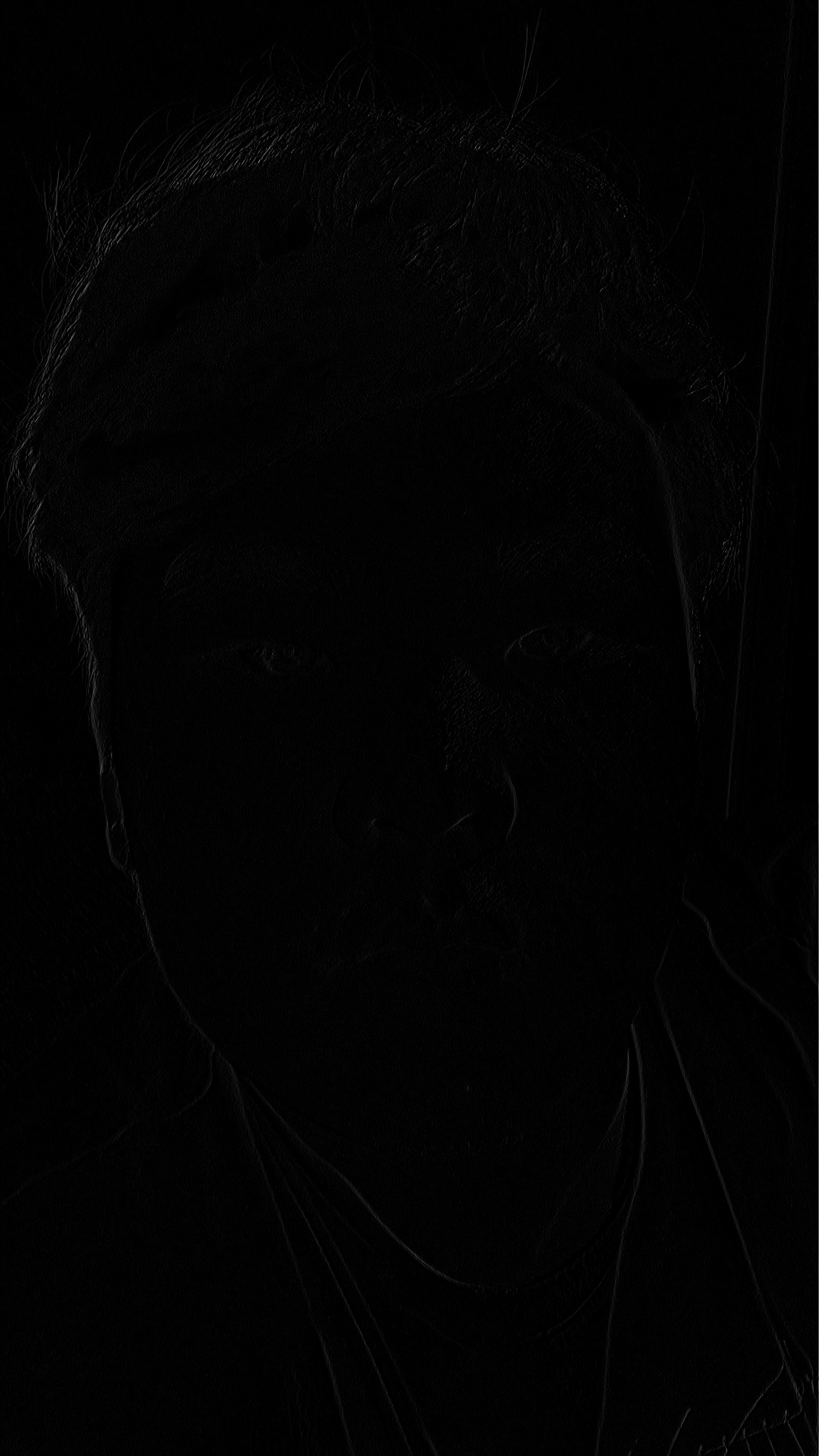
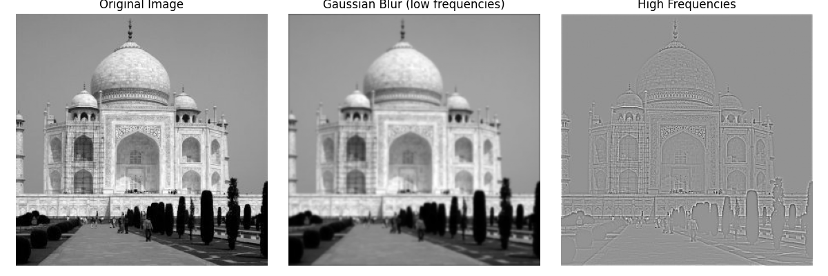
To get the low and high frequencies, we can use a gaussian filter to get the lower frequencies as the higher frequencies will be lost to the filter and then subtract it from the original to get the remaining frequencies, which will be the high frequencies.
The following shows the above process on the Taj Mahal:
We can see the output of various values of alpha:
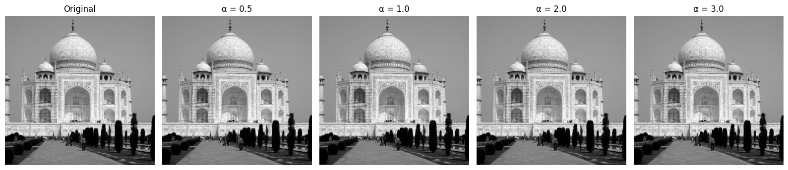
We can see that the output is much sharper when alpha is larger.
To get a hybrid image, the steps go as follows:
To get the low and high frequencies, we can use a gaussian filter to get the lower frequencies as the higher frequencies will be lost to the filter and then subtract it from the original to get the remaining frequencies, which will be the high frequencies.
Here is the output of the hybrid image creation with various steps included:
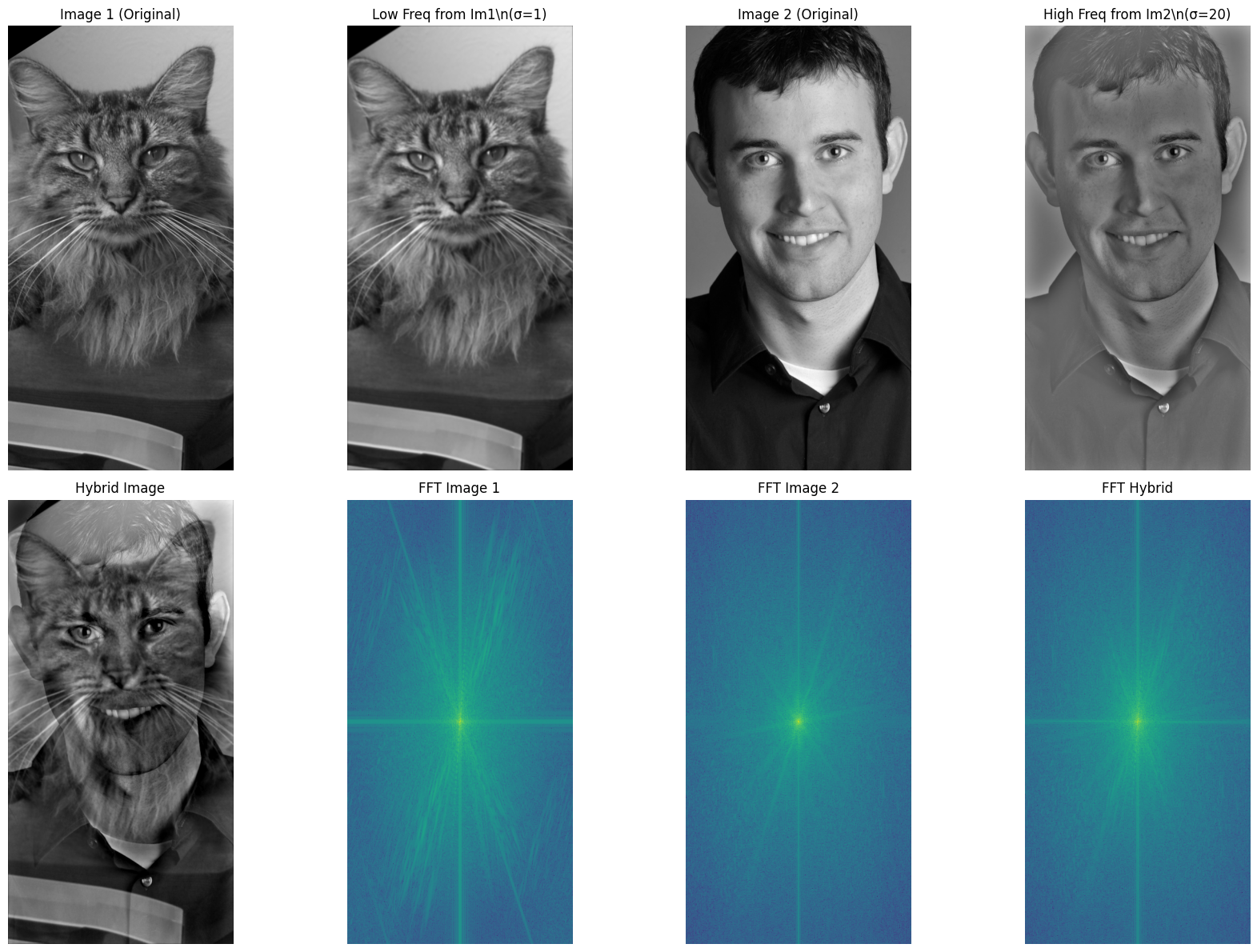
You can see that the FFT of the hybrid is equal to the sum/average of the FFT of the two images.
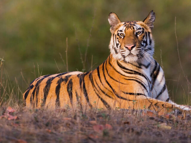
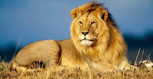
Here are some other hybrid images created from different source pairs:
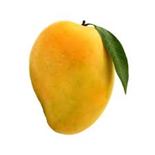
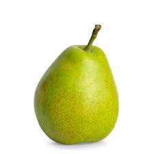
Original source images:
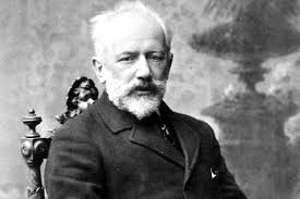
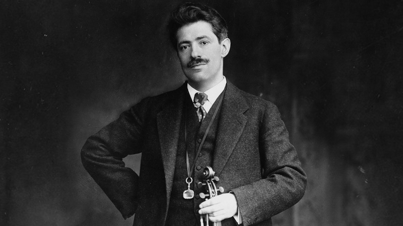
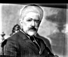
Original source images:
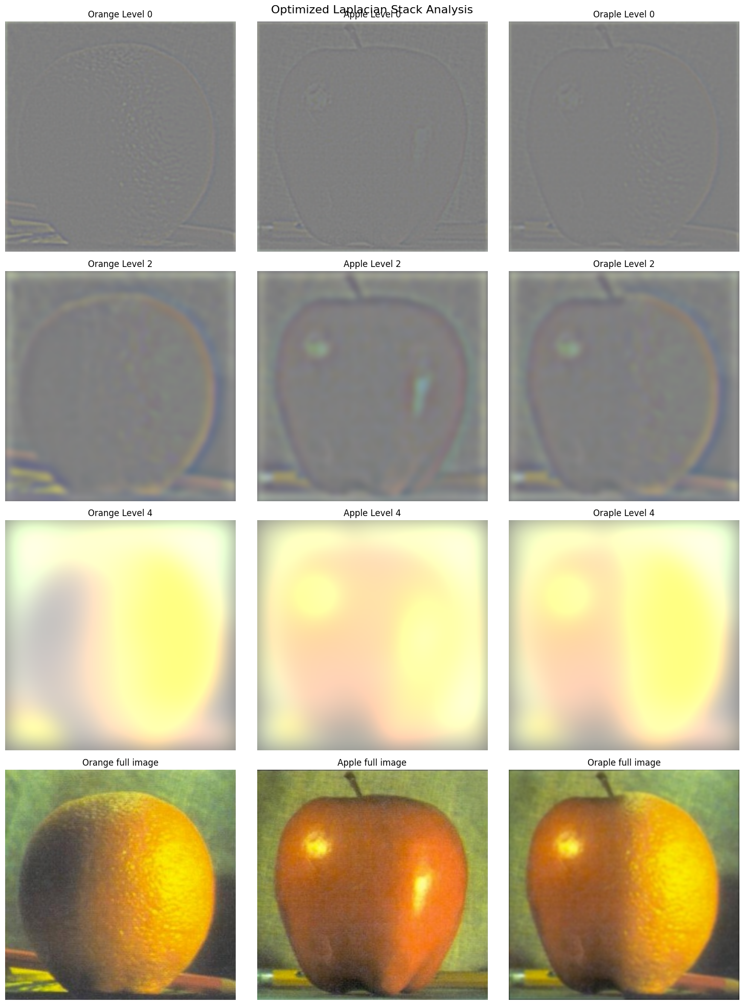
Here is the process of the multiresolution blending using Gaussian and Laplacian stacks:
Original source images:
The multiresolution blending technique allows for seamless combination of images by working in different frequency bands. High frequencies are blended sharply while low frequencies transition smoothly, creating natural-looking results without visible seams.